Deeplearning.ai 笔记作业（一）week4

第一章神经网络和深度学习 week4

笔记

L层深层神经网络

如下图就是一个深层神经网络，相比而言，逻辑回归就是一个浅层的神经网络。
L层深层神经网络

L表示神经网络的层数，L=4，n^[1]=5，n^[2]=5，n^[3]=3，n^[4]=1

a^[L] = activation in Layer L
a^[L] = g^[L](z^[L])，W^[L]= weight for Z^[L]

神经网络的前向传播

就如上图所示：

Input: a^[l-1]
Output: a^[l], z^[l]
notes: 通过神经网络训练过程可以发现，z^[l]在反向传播的过程中也可以利用，所以输出的z^[l]以cache(z^[l])保存

单层计算：
z^[l]=W^[l]a^[l-1]+b^[l]
a^[l]=g^[l](z^[l])

矢量化计算：
Z^[l]=W^[l]A^[l-1]+b^[l]
A^[l]=g^[l](Z^[l])

矢量化时保证矩阵维度正确（重要）

通过观察得出：
W^[l]: (n^[l], n^[l-1])
b^[l]: (n^[l], 1)
dW^[l]: (n^[l], n^[l-1])
db^[l]: (n^[l], 1)
Z^[l]: (n^[l], m)
A^[l]: (n^[l], m)
dZ^[l]: (n^[l], m)
dA^[l]: (n^[l], m)

前向传播与反向传播

前向传播图示：

反向传播图示：

为什么使用深层表示

以下内容的表达参考自cnblogs

直观理解深层网络。

直观理解深层网络
上图所示是一个人脸识别的过程，具体的实现步骤如下：

通过深层神经网络首先会选取一些边缘信息，例如脸形，眼框，总之是一些边框之类的信息(我自己的理解是之所以先找出边缘信息是为了将要观察的事物与周围环境分割开来)，这也就是第一层的作用。
找到边缘信息后，开始放大，将信息聚合在一起。例如找到眼睛轮廓信息后，通过往上一层汇聚从而得到眼睛的信息；同理通过汇聚脸的轮廓信息得到脸颊信息等等
在第二步的基础上将各个局部信息(眼睛、眉毛……)汇聚成一张人脸，最终达到人脸识别的效果。

同样的过程也可以用来表示声音识别过程：一个声音分割成一个一个的片段，然后再选取单个发音（例如C,A,T），然后再组合成单词（CAT），最后在聚合成一个句子或单词。

为什么用深层神经网络而不用浅层神经网络

有一个电路原理，就是说由小的网络单元组成的深层电路往往比浅层电路需要更多的元器件。
比如X₁XOR X₂XOR X₃XOR…X_n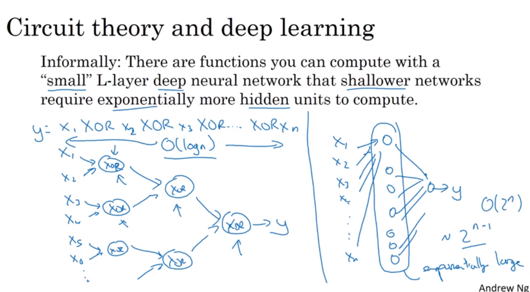

如果是深层网络，只需要O(logn)的数量级，但是如果使用浅层网络的话，就需要遍历所有的情况设置真值表，需要O(2^n-1)。转化成神经网络，要达到相同的目的，浅层网络需要比深层网络更多地神经元个数。

构建深层神经网络块

前向传播：

反向传播：

标准流程：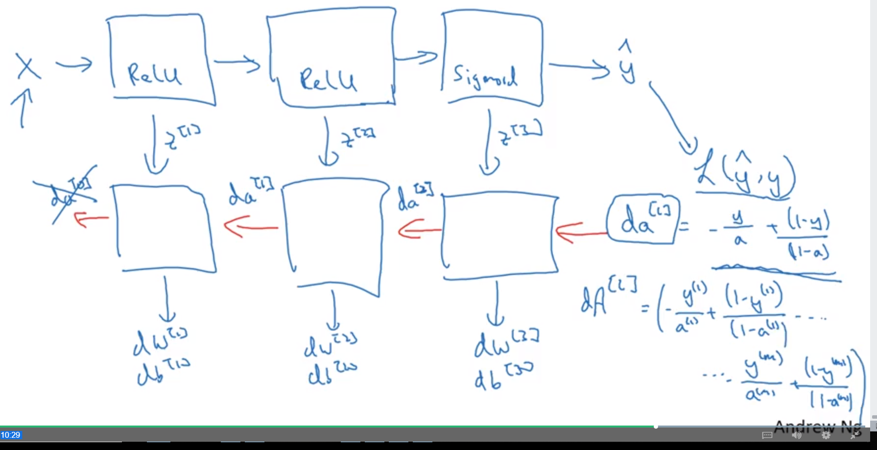
整个流程

参数与超参数

参数：W^[l]，b^[l]
超参数：

学习速率
迭代次数
隐藏层数
神经元个数
激活函数的选择
minibatch size
正则化方法
momentum

所以，对于资深的算法工程师，随着计算资源的不断迭代，适时调整自己的超参数可能会取得更好地结果。

作业

课堂的小quiz可以点击下载

Building your Deep Neural Network: Step by Step

Welcome to your week 4 assignment (part 1 of 2)! You have previously trained a 2-layer Neural Network (with a single hidden layer). This week, you will build a deep neural network, with as many layers as you want!

In this notebook, you will implement all the functions required to build a deep neural network.
In the next assignment, you will use these functions to build a deep neural network for image classification.

After this assignment you will be able to:

Use non-linear units like ReLU to improve your model
Build a deeper neural network (with more than 1 hidden layer)
Implement an easy-to-use neural network class

Notation:

Superscript $[l]$ denotes a quantity associated with the $l^{th}$ layer.
- Example: $a^{[L]}$ is the $L^{th}$ layer activation. $W^{[L]}$ and $b^{[L]}$ are the $L^{th}$ layer parameters.
Superscript $(i)$ denotes a quantity associated with the $i^{th}$ example.
- Example: $x^{(i)}$ is the $i^{th}$ training example.
Lowerscript $i$ denotes the $i^{th}$ entry of a vector.
- Example: $a^{[l]}_i$ denotes the $i^{th}$ entry of the $l^{th}$ layer’s activations).

Let’s get started!

1 - Packages

Let’s first import all the packages that you will need during this assignment.

numpy is the main package for scientific computing with Python.
matplotlib is a library to plot graphs in Python.
dnn_utils provides some necessary functions for this notebook.
testCases provides some test cases to assess the correctness of your functions
np.random.seed(1) is used to keep all the random function calls consistent. It will help us grade your work. Please don’t change the seed.

import numpy as np
import h5py
import matplotlib.pyplot as plt
from testCases_v4 import *
from dnn_utils_v2 import sigmoid, sigmoid_backward, relu, relu_backward

%matplotlib inline
plt.rcParams['figure.figsize'] = (5.0, 4.0) # set default size of plots
plt.rcParams['image.interpolation'] = 'nearest'
plt.rcParams['image.cmap'] = 'gray'

%load_ext autoreload
%autoreload 2

np.random.seed(1)

/opt/conda/lib/python3.5/site-packages/matplotlib/font_manager.py:273: UserWarning: Matplotlib is building the font cache using fc-list. This may take a moment.
  warnings.warn('Matplotlib is building the font cache using fc-list. This may take a moment.')
/opt/conda/lib/python3.5/site-packages/matplotlib/font_manager.py:273: UserWarning: Matplotlib is building the font cache using fc-list. This may take a moment.
  warnings.warn('Matplotlib is building the font cache using fc-list. This may take a moment.')

2 - Outline of the Assignment

To build your neural network, you will be implementing several “helper functions”. These helper functions will be used in the next assignment to build a two-layer neural network and an L-layer neural network. Each small helper function you will implement will have detailed instructions that will walk you through the necessary steps. Here is an outline of this assignment, you will:

Initialize the parameters for a two-layer network and for an $L$-layer neural network.
Implement the forward propagation module (shown in purple in the figure below).
- Complete the LINEAR part of a layer’s forward propagation step (resulting in $Z^{[l]}$).
- We give you the ACTIVATION function (relu/sigmoid).
- Combine the previous two steps into a new [LINEAR->ACTIVATION] forward function.
- Stack the [LINEAR->RELU] forward function L-1 time (for layers 1 through L-1) and add a [LINEAR->SIGMOID] at the end (for the final layer $L$). This gives you a new L_model_forward function.
Compute the loss.
Implement the backward propagation module (denoted in red in the figure below).
- Complete the LINEAR part of a layer’s backward propagation step.
- We give you the gradient of the ACTIVATE function (relu_backward/sigmoid_backward)
- Combine the previous two steps into a new [LINEAR->ACTIVATION] backward function.
- Stack [LINEAR->RELU] backward L-1 times and add [LINEAR->SIGMOID] backward in a new L_model_backward function
Finally update the parameters.

Figure 1

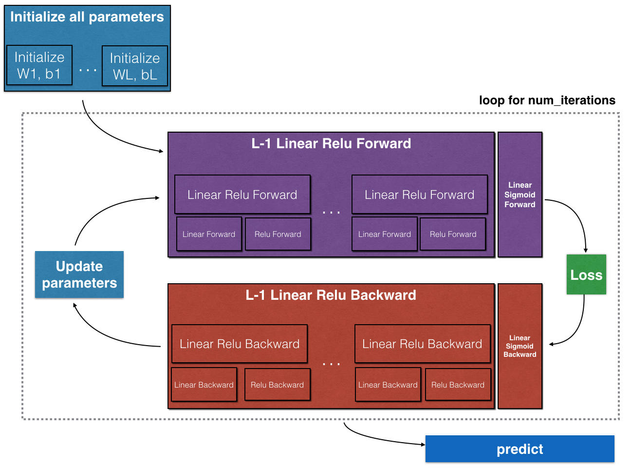
Note that for every forward function, there is a corresponding backward function. That is why at every step of your forward module you will be storing some values in a cache. The cached values are useful for computing gradients. In the backpropagation module you will then use the cache to calculate the gradients. This assignment will show you exactly how to carry out each of these steps.

#### 3 - Initialization

You will write two helper functions that will initialize the parameters for your model. The first function will be used to initialize parameters for a two layer model. The second one will generalize this initialization process to $L$ layers.

##### 3.1 - 2-layer Neural Network

Exercise: Create and initialize the parameters of the 2-layer neural network.

Instructions:
- The model’s structure is: LINEAR -> RELU -> LINEAR -> SIGMOID.
- Use random initialization for the weight matrices. Use np.random.randn(shape)*0.01 with the correct shape.
- Use zero initialization for the biases. Use np.zeros(shape).

# GRADED FUNCTION: initialize_parameters

def initialize_parameters(n_x, n_h, n_y):
    """
    Argument:
    n_x -- size of the input layer
    n_h -- size of the hidden layer
    n_y -- size of the output layer
    
    Returns:
    parameters -- python dictionary containing your parameters:
                    W1 -- weight matrix of shape (n_h, n_x)
                    b1 -- bias vector of shape (n_h, 1)
                    W2 -- weight matrix of shape (n_y, n_h)
                    b2 -- bias vector of shape (n_y, 1)
    """
    
    np.random.seed(1)
    
    ### START CODE HERE ### (≈ 4 lines of code)
    # random不要用元组, zeros用元组
    W1 = np.random.randn(n_h, n_x) * 0.01
    b1 = np.zeros((n_h, 1))
    W2 = np.random.randn(n_y, n_h) * 0.01
    b2 = np.zeros((n_y, 1))
    ### END CODE HERE ###
    
    assert(W1.shape == (n_h, n_x))
    assert(b1.shape == (n_h, 1))
    assert(W2.shape == (n_y, n_h))
    assert(b2.shape == (n_y, 1))
    
    parameters = &#123;"W1": W1,
                  "b1": b1,
                  "W2": W2,
                  "b2": b2&#125;
    
    return parameters

parameters = initialize_parameters(3,2,1)
print("W1 = " + str(parameters["W1"]))
print("b1 = " + str(parameters["b1"]))
print("W2 = " + str(parameters["W2"]))
print("b2 = " + str(parameters["b2"]))

W1 = [[ 0.01624345 -0.00611756 -0.00528172]
[-0.01072969 0.00865408 -0.02301539]]
b1 = [[ 0.]
[ 0.]]
W2 = [[ 0.01744812 -0.00761207]]
b2 = [[ 0.]]

Expected output:

W1	[[ 0.01624345 -0.00611756 -0.00528172] [-0.01072969 0.00865408 -0.02301539]]
b1	[[ 0.] [ 0.]]
W2	[[ 0.01744812 -0.00761207]]
b2	[[ 0.]]

##### 3.2 - L-layer Neural Network

The initialization for a deeper L-layer neural network is more complicated because there are many more weight matrices and bias vectors. When completing the initialize_parameters_deep, you should make sure that your dimensions match between each layer. Recall that $n^{[l]}$ is the number of units in layer $l$. Thus for example if the size of our input $X$ is $(12288, 209)$ (with $m=209$ examples) then:

	Shape of W	Shape of b	Activation	Shape of Activation
Layer 1	$(n^{[1]},12288)$	$(n^{[1]},1)$	$Z^{[1]} = W^{[1]} X + b^{[1]} $	$(n^{[1]},209)$
Layer 2	$(n^{[2]}, n^{[1]})$	$(n^{[2]},1)$	$Z^{[2]} = W^{[2]} A^{[1]} + b^{[2]}$	$(n^{[2]}, 209)$
$\vdots$	$\vdots$	$\vdots$	$\vdots$	$\vdots$
Layer L-1	$(n^{[L-1]}, n^{[L-2]})$	$(n^{[L-1]}, 1)$	$Z^{[L-1]} = W^{[L-1]} A^{[L-2]} + b^{[L-1]}$	$(n^{[L-1]}, 209)$
Layer L	$(n^{[L]}, n^{[L-1]})$	$(n^{[L]}, 1)$	$Z^{[L]} = W^{[L]} A^{[L-1]} + b^{[L]}$	$(n^{[L]}, 209)$

Remember that when we compute $W X + b$ in python, it carries out broadcasting. For example, if:

$$ W = \begin{bmatrix}
j & k & l\\
m & n & o \\
p & q & r
\end{bmatrix}\;\;\; X = \begin{bmatrix}
a & b & c\\
d & e & f \\
g & h & i
\end{bmatrix} \;\;\; b =\begin{bmatrix}
s \\
t \\
u
\end{bmatrix}\tag{2}$$

Then $WX + b$ will be:

$$ WX + b = \begin{bmatrix}
(ja + kd + lg) + s & (jb + ke + lh) + s & (jc + kf + li)+ s\\
(ma + nd + og) + t & (mb + ne + oh) + t & (mc + nf + oi) + t\\
(pa + qd + rg) + u & (pb + qe + rh) + u & (pc + qf + ri)+ u
\end{bmatrix}\tag{3} $$

Exercise: Implement initialization for an L-layer Neural Network.

Instructions:
- The model’s structure is [LINEAR -> RELU] $ \times$ (L-1) -> LINEAR -> SIGMOID. I.e., it has $L-1$ layers using a ReLU activation function followed by an output layer with a sigmoid activation function.
- Use random initialization for the weight matrices. Use np.random.randn(shape) * 0.01.
- Use zeros initialization for the biases. Use np.zeros(shape).
- We will store $n^{[l]}$, the number of units in different layers, in a variable layer_dims. For example, the layer_dims for the “Planar Data classification model” from last week would have been [2,4,1]: There were two inputs, one hidden layer with 4 hidden units, and an output layer with 1 output unit. Thus means W1‘s shape was (4,2), b1 was (4,1), W2 was (1,4) and b2 was (1,1). Now you will generalize this to $L$ layers!
- Here is the implementation for $L=1$ (one layer neural network). It should inspire you to implement the general case (L-layer neural network).

1
2
3

if L == 1:
    parameters["W" + str(L)] = np.random.randn(layer_dims[1], layer_dims[0]) * 0.01
    parameters["b" + str(L)] = np.zeros((layer_dims[1], 1))

# GRADED FUNCTION: initialize_parameters_deep

def initialize_parameters_deep(layer_dims):
    """
    Arguments:
    layer_dims -- python array (list) containing the dimensions of each layer in our network
    
    Returns:
    parameters -- python dictionary containing your parameters "W1", "b1", ..., "WL", "bL":
                    Wl -- weight matrix of shape (layer_dims[l], layer_dims[l-1])
                    bl -- bias vector of shape (layer_dims[l], 1)
    """
    
    np.random.seed(3)
    parameters = &#123;&#125;
    L = len(layer_dims)            # number of layers in the network

    for l in range(1, L):
        ### START CODE HERE ### (≈ 2 lines of code)
        parameters['W' + str(l)] = np.random.randn(layer_dims[l], layer_dims[l-1]) * 0.01
        parameters['b' + str(l)] = np.zeros((layer_dims[l], 1))
        ### END CODE HERE ###
        
        assert(parameters['W' + str(l)].shape == (layer_dims[l], layer_dims[l-1]))
        assert(parameters['b' + str(l)].shape == (layer_dims[l], 1))

        
    return parameters

parameters = initialize_parameters_deep([5,4,3])
print("W1 = " + str(parameters["W1"]))
print("b1 = " + str(parameters["b1"]))
print("W2 = " + str(parameters["W2"]))
print("b2 = " + str(parameters["b2"]))

W1 = [[ 0.01788628 0.0043651 0.00096497 -0.01863493 -0.00277388]
[-0.00354759 -0.00082741 -0.00627001 -0.00043818 -0.00477218]
[-0.01313865 0.00884622 0.00881318 0.01709573 0.00050034]
[-0.00404677 -0.0054536 -0.01546477 0.00982367 -0.01101068]]
b1 = [[ 0.]
[ 0.]
[ 0.]
[ 0.]]
W2 = [[-0.01185047 -0.0020565 0.01486148 0.00236716]
[-0.01023785 -0.00712993 0.00625245 -0.00160513]
[-0.00768836 -0.00230031 0.00745056 0.01976111]]
b2 = [[ 0.]
[ 0.]
[ 0.]]

Expected output:

W1	[[ 0.01788628 0.0043651 0.00096497 -0.01863493 -0.00277388] [-0.00354759 -0.00082741 -0.00627001 -0.00043818 -0.00477218] [-0.01313865 0.00884622 0.00881318 0.01709573 0.00050034] [-0.00404677 -0.0054536 -0.01546477 0.00982367 -0.01101068]]
b1	[[ 0.] [ 0.] [ 0.] [ 0.]]
W2	[[-0.01185047 -0.0020565 0.01486148 0.00236716] [-0.01023785 -0.00712993 0.00625245 -0.00160513] [-0.00768836 -0.00230031 0.00745056 0.01976111]]
b2	[[ 0.] [ 0.] [ 0.]]

#### 4 - Forward propagation module

##### 4.1 - Linear Forward
Now that you have initialized your parameters, you will do the forward propagation module. You will start by implementing some basic functions that you will use later when implementing the model. You will complete three functions in this order:

- LINEAR
- LINEAR -> ACTIVATION where ACTIVATION will be either ReLU or Sigmoid.
- [LINEAR -> RELU] $\times$ (L-1) -> LINEAR -> SIGMOID (whole model)

The linear forward module (vectorized over all the examples) computes the following equations:

$$Z^{[l]} = W^{[l]}A^{[l-1]} +b^{[l]}\tag{4}$$

where $A^{[0]} = X$.

Exercise: Build the linear part of forward propagation.

Reminder:
The mathematical representation of this unit is $Z^{[l]} = W^{[l]}A^{[l-1]} +b^{[l]}$. You may also find np.dot() useful. If your dimensions don’t match, printing W.shape may help.

# GRADED FUNCTION: linear_forward

def linear_forward(A, W, b):
    """
    Implement the linear part of a layer's forward propagation.

    Arguments:
    A -- activations from previous layer (or input data): (size of previous layer, number of examples)
    W -- weights matrix: numpy array of shape (size of current layer, size of previous layer)
    b -- bias vector, numpy array of shape (size of the current layer, 1)

    Returns:
    Z -- the input of the activation function, also called pre-activation parameter 
    cache -- a python dictionary containing "A", "W" and "b" ; stored for computing the backward pass efficiently
    """
    
    ### START CODE HERE ### (≈ 1 line of code)
    Z = np.dot(W, A) + b
    ### END CODE HERE ###
    
    assert(Z.shape == (W.shape[0], A.shape[1]))
    cache = (A, W, b)
    
    return Z, cache

A, W, b = linear_forward_test_case()

Z, linear_cache = linear_forward(A, W, b)
print("Z = " + str(Z))

Z = [[ 3.26295337 -1.23429987]]

Expected output:

Z	[[ 3.26295337 -1.23429987]]

##### 4.2 - Linear-Activation Forward

In this notebook, you will use two activation functions:

- Sigmoid: $\sigma(Z) = \sigma(W A + b) = \frac{1}{ 1 + e^{-(W A + b)}}$. We have provided you with the sigmoid function. This function returns two items: the activation value “a“ and a “cache“ that contains “Z“ (it’s what we will feed in to the corresponding backward function). To use it you could just call:

1	A, activation_cache = sigmoid(Z)

- ReLU: The mathematical formula for ReLu is $A = RELU(Z) = max(0, Z)$. We have provided you with the relu function. This function returns two items: the activation value “A“ and a “cache“ that contains “Z“ (it’s what we will feed in to the corresponding backward function). To use it you could just call:

1	A, activation_cache = relu(Z)

For more convenience, you are going to group two functions (Linear and Activation) into one function (LINEAR->ACTIVATION). Hence, you will implement a function that does the LINEAR forward step followed by an ACTIVATION forward step.

Exercise: Implement the forward propagation of the LINEAR->ACTIVATION layer. Mathematical relation is: $A^{[l]} = g(Z^{[l]}) = g(W^{[l]}A^{[l-1]} +b^{[l]})$ where the activation “g” can be sigmoid() or relu(). Use linear_forward() and the correct activation function.

# GRADED FUNCTION: linear_activation_forward

def linear_activation_forward(A_prev, W, b, activation):
    """
    Implement the forward propagation for the LINEAR->ACTIVATION layer

    Arguments:
    A_prev -- activations from previous layer (or input data): (size of previous layer, number of examples)
    W -- weights matrix: numpy array of shape (size of current layer, size of previous layer)
    b -- bias vector, numpy array of shape (size of the current layer, 1)
    activation -- the activation to be used in this layer, stored as a text string: "sigmoid" or "relu"

    Returns:
    A -- the output of the activation function, also called the post-activation value 
    cache -- a python dictionary containing "linear_cache" and "activation_cache";
             stored for computing the backward pass efficiently
    """
    
    if activation == "sigmoid":
        # Inputs: "A_prev, W, b". Outputs: "A, activation_cache".
        ### START CODE HERE ### (≈ 2 lines of code)
        Z, linear_cache = linear_forward(A_prev, W, b)
        A, activation_cache = sigmoid(Z)
        ### END CODE HERE ###
    
    elif activation == "relu":
        # Inputs: "A_prev, W, b". Outputs: "A, activation_cache".
        ### START CODE HERE ### (≈ 2 lines of code)
        Z, linear_cache = linear_forward(A_prev, W, b)
        A, activation_cache = relu(Z)
        ### END CODE HERE ###
    
    assert (A.shape == (W.shape[0], A_prev.shape[1]))
    cache = (linear_cache, activation_cache)

    return A, cache

A_prev, W, b = linear_activation_forward_test_case()

A, linear_activation_cache = linear_activation_forward(A_prev, W, b, activation = "sigmoid")
print("With sigmoid: A = " + str(A))

A, linear_activation_cache = linear_activation_forward(A_prev, W, b, activation = "relu")
print("With ReLU: A = " + str(A))

With sigmoid: A = [[ 0.96890023 0.11013289]]
With ReLU: A = [[ 3.43896131 0. ]]

Expected output:

With sigmoid: A	[[ 0.96890023 0.11013289]]
With ReLU: A	[[ 3.43896131 0. ]]

Note: In deep learning, the “[LINEAR->ACTIVATION]” computation is counted as a single layer in the neural network, not two layers.

##### d) L-Layer Model

For even more convenience when implementing the $L$-layer Neural Net, you will need a function that replicates the previous one (linear_activation_forward with RELU) $L-1$ times, then follows that with one linear_activation_forward with SIGMOID.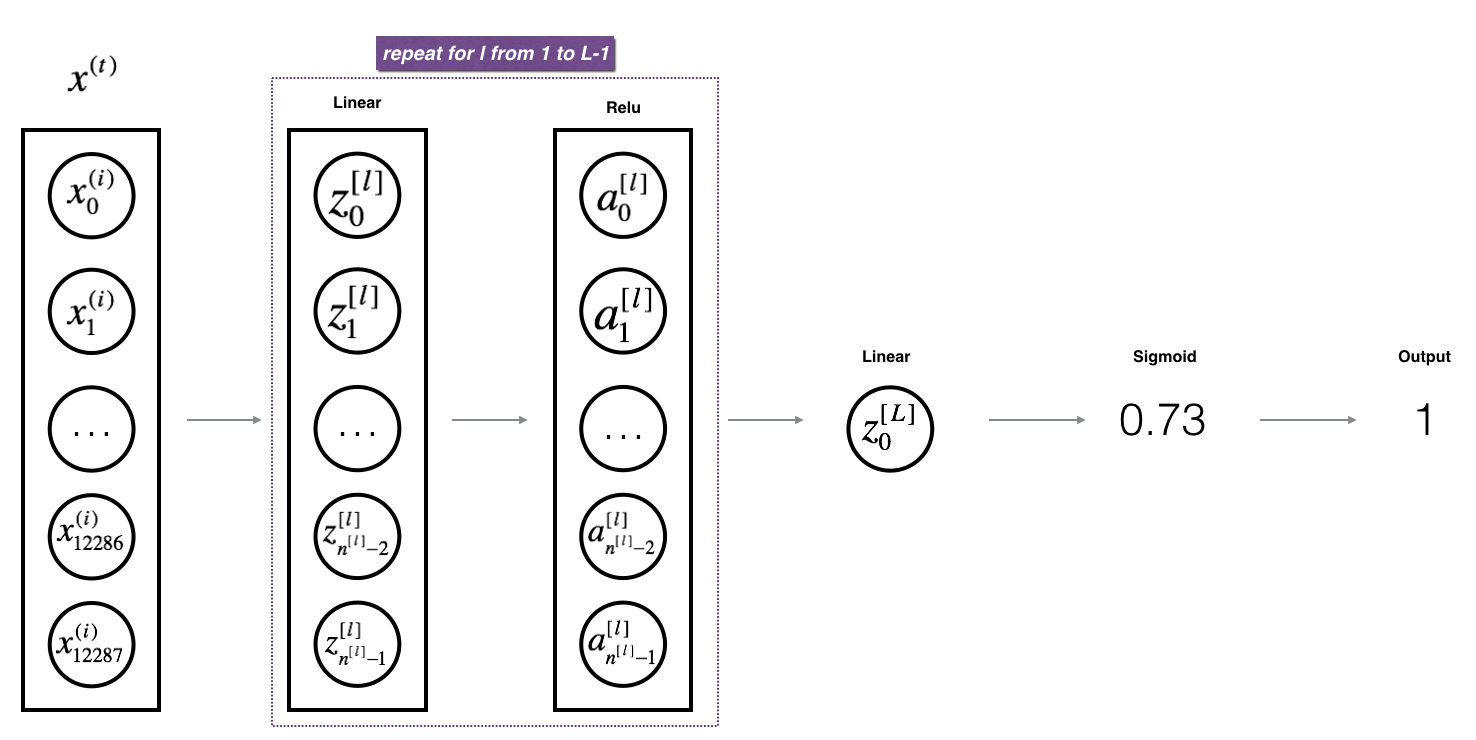

Figure 2 : [LINEAR -> RELU] $\times$ (L-1) -> LINEAR -> SIGMOID model

Exercise: Implement the forward propagation of the above model.

Instruction: In the code below, the variable AL will denote $A^{[L]} = \sigma(Z^{[L]}) = \sigma(W^{[L]} A^{[L-1]} + b^{[L]})$. (This is sometimes also called Yhat, i.e., this is $\hat{Y}$.)

Tips:
- Use the functions you had previously written
- Use a for loop to replicate [LINEAR->RELU] (L-1) times
- Don’t forget to keep track of the caches in the “caches” list. To add a new value c to a list, you can use list.append(c).

# GRADED FUNCTION: L_model_forward

def L_model_forward(X, parameters):
    """
    Implement forward propagation for the [LINEAR->RELU]*(L-1)->LINEAR->SIGMOID computation
    
    Arguments:
    X -- data, numpy array of shape (input size, number of examples)
    parameters -- output of initialize_parameters_deep()
    
    Returns:
    AL -- last post-activation value
    caches -- list of caches containing:
                every cache of linear_activation_forward() (there are L-1 of them, indexed from 0 to L-1)
    """

    caches = []
    A = X
    L = len(parameters) // 2                  # number of layers in the neural network
    
    # Implement [LINEAR -> RELU]*(L-1). Add "cache" to the "caches" list.
    for l in range(1, L):
        A_prev = A 
        ### START CODE HERE ### (≈ 2 lines of code)
        A, cache = linear_activation_forward(A_prev, parameters["W" + str(l)], parameters["b" + str(l)], "relu")
        caches.append(cache)
        ### END CODE HERE ###
    
    # Implement LINEAR -> SIGMOID. Add "cache" to the "caches" list.
    ### START CODE HERE ### (≈ 2 lines of code)
    AL, cache = linear_activation_forward(A, parameters["W" + str(L)], parameters["b" + str(L)], "sigmoid")
    caches.append(cache)
    ### END CODE HERE ###
    
    assert(AL.shape == (1,X.shape[1]))
            
    return AL, caches

X, parameters = L_model_forward_test_case_2hidden()
AL, caches = L_model_forward(X, parameters)
print("AL = " + str(AL))
print("Length of caches list = " + str(len(caches)))

AL = [[ 0.03921668 0.70498921 0.19734387 0.04728177]]
Length of caches list = 3

AL	[[ 0.03921668 0.70498921 0.19734387 0.04728177]]
Length of caches list	3

Great! Now you have a full forward propagation that takes the input X and outputs a row vector $A^{[L]}$ containing your predictions. It also records all intermediate values in “caches”. Using $A^{[L]}$, you can compute the cost of your predictions.

#### 5 - Cost function

Now you will implement forward and backward propagation. You need to compute the cost, because you want to check if your model is actually learning.

Exercise: Compute the cross-entropy cost $J$, using the following formula: $$-\frac{1}{m} \sum\limits_{i = 1}^{m} (y^{(i)}\log\left(a^{[L] (i)}\right) + (1-y^{(i)})\log\left(1- a^{L}\right)) \tag{7}$$

# GRADED FUNCTION: compute_cost

def compute_cost(AL, Y):
    """
    Implement the cost function defined by equation (7).

    Arguments:
    AL -- probability vector corresponding to your label predictions, shape (1, number of examples)
    Y -- true "label" vector (for example: containing 0 if non-cat, 1 if cat), shape (1, number of examples)

    Returns:
    cost -- cross-entropy cost
    """
    
    m = Y.shape[1]

    # Compute loss from aL and y.
    ### START CODE HERE ### (≈ 1 lines of code)
    cost = np.sum(np.multiply(np.log(AL),Y) + np.multiply(np.log(1 - AL), 1 - Y)) / (-m)
    ### END CODE HERE ###
    
    cost = np.squeeze(cost)      # To make sure your cost's shape is what we expect (e.g. this turns [[17]] into 17).
    assert(cost.shape == ())
    
    return cost

1
2
3

Y, AL = compute_cost_test_case()

print("cost = " + str(compute_cost(AL, Y)))

cost = 0.414931599615

Expected Output:

cost

0.41493159961539694

#### 6 - Backward propagation module

Just like with forward propagation, you will implement helper functions for backpropagation. Remember that back propagation is used to calculate the gradient of the loss function with respect to the parameters.

Reminder:

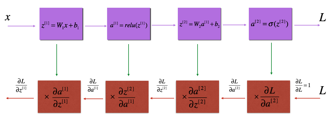
Figure 3 : Forward and Backward propagation for LINEAR->RELU->LINEAR->SIGMOID
The purple blocks represent the forward propagation, and the red blocks represent the backward propagation.

Now, similar to forward propagation, you are going to build the backward propagation in three steps:

LINEAR backward
LINEAR -> ACTIVATION backward where ACTIVATION computes the derivative of either the ReLU or sigmoid activation
[LINEAR -> RELU] $\times$ (L-1) -> LINEAR -> SIGMOID backward (whole model)

6.1 - Linear backward

For layer $l$, the linear part is: $Z^{[l]} = W^{[l]} A^{[l-1]} + b^{[l]}$ (followed by an activation).

Suppose you have already calculated the derivative $dZ^{[l]} = \frac{\partial \mathcal{L} }{\partial Z^{[l]}}$. You want to get $(dW^{[l]}, db^{[l]} dA^{[l-1]})$.

Figure 4

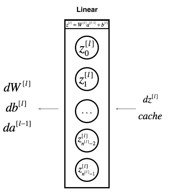
The three outputs $(dW^{[l]}, db^{[l]}, dA^{[l]})$ are computed using the input $dZ^{[l]}$.Here are the formulas you need:
$$ dW^{[l]} = \frac{\partial \mathcal{L} }{\partial W^{[l]}} = \frac{1}{m} dZ^{[l]} A^{[l-1] T} \tag{8}$$
$$ db^{[l]} = \frac{\partial \mathcal{L} }{\partial b^{[l]}} = \frac{1}{m} \sum_{i = 1}^{m} dZ^{l}\tag{9}$$
$$ dA^{[l-1]} = \frac{\partial \mathcal{L} }{\partial A^{[l-1]}} = W^{[l] T} dZ^{[l]} \tag{10}$$

Exercise: Use the 3 formulas above to implement linear_backward().

# GRADED FUNCTION: linear_backward

def linear_backward(dZ, cache):
    """
    Implement the linear portion of backward propagation for a single layer (layer l)

    Arguments:
    dZ -- Gradient of the cost with respect to the linear output (of current layer l)
    cache -- tuple of values (A_prev, W, b) coming from the forward propagation in the current layer

    Returns:
    dA_prev -- Gradient of the cost with respect to the activation (of the previous layer l-1), same shape as A_prev
    dW -- Gradient of the cost with respect to W (current layer l), same shape as W
    db -- Gradient of the cost with respect to b (current layer l), same shape as b
    """
    A_prev, W, b = cache
    m = A_prev.shape[1]

    ### START CODE HERE ### (≈ 3 lines of code)
    dW = np.dot(dZ, A_prev.T) / m
    db = np.sum(dZ, axis=1, keepdims=True) / m
    dA_prev = np.dot(W.T, dZ)
    ### END CODE HERE ###
    
    assert (dA_prev.shape == A_prev.shape)
    assert (dW.shape == W.shape)
    assert (db.shape == b.shape)
    
    return dA_prev, dW, db

# Set up some test inputs
dZ, linear_cache = linear_backward_test_case()

dA_prev, dW, db = linear_backward(dZ, linear_cache)
print ("dA_prev = "+ str(dA_prev))
print ("dW = " + str(dW))
print ("db = " + str(db))

dA_prev = [[ 0.51822968 -0.19517421]
 [-0.40506361  0.15255393]
 [ 2.37496825 -0.89445391]]
dW = [[-0.10076895  1.40685096  1.64992505]]
db = [[ 0.50629448]]

Expected Output:

dA_prev	[[ 0.51822968 -0.19517421] [-0.40506361 0.15255393] [ 2.37496825 -0.89445391]]
dW	[[-0.10076895 1.40685096 1.64992505]]
db	[[ 0.50629448]]

6.2 - Linear-Activation backward

Next, you will create a function that merges the two helper functions: linear_backward and the backward step for the activation linear_activation_backward.

To help you implement linear_activation_backward, we provided two backward functions:

sigmoid_backward: Implements the backward propagation for SIGMOID unit. You can call it as follows:

1	dZ = sigmoid_backward(dA, activation_cache)

relu_backward: Implements the backward propagation for RELU unit. You can call it as follows:

1	dZ = relu_backward(dA, activation_cache)

If $g(.)$ is the activation function,
sigmoid_backward and relu_backward compute $$dZ^{[l]} = dA^{[l]} * g’(Z^{[l]}) \tag{11}$$.

Exercise: Implement the backpropagation for the LINEAR->ACTIVATION layer.

# GRADED FUNCTION: linear_activation_backward

def linear_activation_backward(dA, cache, activation):
    """
    Implement the backward propagation for the LINEAR->ACTIVATION layer.
    
    Arguments:
    dA -- post-activation gradient for current layer l 
    cache -- tuple of values (linear_cache, activation_cache) we store for computing backward propagation efficiently
    activation -- the activation to be used in this layer, stored as a text string: "sigmoid" or "relu"
    
    Returns:
    dA_prev -- Gradient of the cost with respect to the activation (of the previous layer l-1), same shape as A_prev
    dW -- Gradient of the cost with respect to W (current layer l), same shape as W
    db -- Gradient of the cost with respect to b (current layer l), same shape as b
    """
    linear_cache, activation_cache = cache
    
    if activation == "relu":
        ### START CODE HERE ### (≈ 2 lines of code)
        dZ = relu_backward(dA, activation_cache)
        dA_prev, dW, db = linear_backward(dZ, linear_cache)
        ### END CODE HERE ###

    elif activation == "sigmoid":
        ### START CODE HERE ### (≈ 2 lines of code)
        dZ = sigmoid_backward(dA, activation_cache)
        dA_prev, dW, db = linear_backward(dZ, linear_cache)
        ### END CODE HERE ###
    
    return dA_prev, dW, db

dAL, linear_activation_cache = linear_activation_backward_test_case()

dA_prev, dW, db = linear_activation_backward(dAL, linear_activation_cache, activation = "sigmoid")
print ("sigmoid:")
print ("dA_prev = "+ str(dA_prev))
print ("dW = " + str(dW))
print ("db = " + str(db) + "\n")

dA_prev, dW, db = linear_activation_backward(dAL, linear_activation_cache, activation = "relu")
print ("relu:")
print ("dA_prev = "+ str(dA_prev))
print ("dW = " + str(dW))
print ("db = " + str(db))

sigmoid:
dA_prev = [[ 0.11017994  0.01105339]
 [ 0.09466817  0.00949723]
 [-0.05743092 -0.00576154]]
dW = [[ 0.10266786  0.09778551 -0.01968084]]
db = [[-0.05729622]]

relu:
dA_prev = [[ 0.44090989  0.        ]
 [ 0.37883606  0.        ]
 [-0.2298228   0.        ]]
dW = [[ 0.44513824  0.37371418 -0.10478989]]
db = [[-0.20837892]]

Expected output with sigmoid:

dA_prev	[[ 0.11017994 0.01105339] [ 0.09466817 0.00949723] [-0.05743092 -0.00576154]]
dW	[[ 0.10266786 0.09778551 -0.01968084]]
db	[[-0.05729622]]

Expected output with relu:

dA_prev	[[ 0.44090989 0. ] [ 0.37883606 0. ] [-0.2298228 0. ]]
dW	[[ 0.44513824 0.37371418 -0.10478989]]
db	[[-0.20837892]]

6.3 - L-Model Backward

Now you will implement the backward function for the whole network. Recall that when you implemented the L_model_forward function, at each iteration, you stored a cache which contains (X,W,b, and z). In the back propagation module, you will use those variables to compute the gradients. Therefore, in the L_model_backward function, you will iterate through all the hidden layers backward, starting from layer $L$. On each step, you will use the cached values for layer $l$ to backpropagate through layer $l$. Figure 5 below shows the backward pass.

Figure 5 : Backward pass

Initializing backpropagation:
To backpropagate through this network, we know that the output is,
$A^{[L]} = \sigma(Z^{[L]})$. Your code thus needs to compute dAL $= \frac{\partial \mathcal{L}}{\partial A^{[L]}}$.
To do so, use this formula (derived using calculus which you don’t need in-depth knowledge of):

1	dAL = - (np.divide(Y, AL) - np.divide(1 - Y, 1 - AL)) # derivative of cost with respect to AL

You can then use this post-activation gradient dAL to keep going backward. As seen in Figure 5, you can now feed in dAL into the LINEAR->SIGMOID backward function you implemented (which will use the cached values stored by the L_model_forward function). After that, you will have to use a for loop to iterate through all the other layers using the LINEAR->RELU backward function. You should store each dA, dW, and db in the grads dictionary. To do so, use this formula :

$$grads[“dW” + str(l)] = dW^{[l]}\tag{15} $$

For example, for $l=3$ this would store $dW^{[l]}$ in grads["dW3"].

Exercise: Implement backpropagation for the [LINEAR->RELU] $\times$ (L-1) -> LINEAR -> SIGMOID model.

# GRADED FUNCTION: L_model_backward

def L_model_backward(AL, Y, caches):
    """
    Implement the backward propagation for the [LINEAR->RELU] * (L-1) -> LINEAR -> SIGMOID group
    
    Arguments:
    AL -- probability vector, output of the forward propagation (L_model_forward())
    Y -- true "label" vector (containing 0 if non-cat, 1 if cat)
    caches -- list of caches containing:
                every cache of linear_activation_forward() with "relu" (it's caches[l], for l in range(L-1) i.e l = 0...L-2)
                the cache of linear_activation_forward() with "sigmoid" (it's caches[L-1])
    
    Returns:
    grads -- A dictionary with the gradients
             grads["dA" + str(l)] = ... 
             grads["dW" + str(l)] = ...
             grads["db" + str(l)] = ... 
    """
    grads = &#123;&#125;
    L = len(caches) # the number of layers
    m = AL.shape[1]
    Y = Y.reshape(AL.shape) # after this line, Y is the same shape as AL
    
    # Initializing the backpropagation
    ### START CODE HERE ### (1 line of code)
    dAL = -(np.divide(Y, AL) - np.divide((1-Y), (1-AL)))
    ### END CODE HERE ###
    
    # Lth layer (SIGMOID -> LINEAR) gradients. Inputs: "dAL, current_cache". Outputs: "grads["dAL-1"], grads["dWL"], grads["dbL"]
    ### START CODE HERE ### (approx. 2 lines)
    current_cache = caches[L - 1]
    grads["dA" + str(L-1)], grads["dW" + str(L)], grads["db" + str(L)] = linear_activation_backward(dAL, current_cache, "sigmoid")
    ### END CODE HERE ###
    
    # Loop from l=L-2 to l=0
    for l in reversed(range(L-1)):
        # lth layer: (RELU -> LINEAR) gradients.
        # Inputs: "grads["dA" + str(l + 1)], current_cache". Outputs: "grads["dA" + str(l)] , grads["dW" + str(l + 1)] , grads["db" + str(l + 1)] 
        ### START CODE HERE ### (approx. 5 lines)
        current_cache = caches[l]
        dA_prev_temp, dW_temp, db_temp = linear_activation_backward(grads["dA" + str(l + 1)], current_cache, "relu")
        grads["dA" + str(l)] = dA_prev_temp
        grads["dW" + str(l + 1)] = dW_temp
        grads["db" + str(l + 1)] = db_temp
        ### END CODE HERE ###

    return grads

1
2
3

AL, Y_assess, caches = L_model_backward_test_case()
grads = L_model_backward(AL, Y_assess, caches)
print_grads(grads)

dW1 = [[ 0.41010002  0.07807203  0.13798444  0.10502167]
 [ 0.          0.          0.          0.        ]
 [ 0.05283652  0.01005865  0.01777766  0.0135308 ]]
db1 = [[-0.22007063]
 [ 0.        ]
 [-0.02835349]]
dA1 = [[ 0.12913162 -0.44014127]
 [-0.14175655  0.48317296]
 [ 0.01663708 -0.05670698]]

Expected Output

dW1	[[ 0.41010002 0.07807203 0.13798444 0.10502167] [ 0. 0. 0. 0. ] [ 0.05283652 0.01005865 0.01777766 0.0135308 ]]
db1	[[-0.22007063] [ 0. ] [-0.02835349]]
dA1	[[ 0.12913162 -0.44014127] [-0.14175655 0.48317296] [ 0.01663708 -0.05670698]]

6.4 - Update Parameters

In this section you will update the parameters of the model, using gradient descent:

$$ W^{[l]} = W^{[l]} - \alpha \text{ } dW^{[l]} \tag{16}$$
$$ b^{[l]} = b^{[l]} - \alpha \text{ } db^{[l]} \tag{17}$$

where $\alpha$ is the learning rate. After computing the updated parameters, store them in the parameters dictionary.

Exercise: Implement update_parameters() to update your parameters using gradient descent.

Instructions:
Update parameters using gradient descent on every $W^{[l]}$ and $b^{[l]}$ for $l = 1, 2, …, L$.

# GRADED FUNCTION: update_parameters

def update_parameters(parameters, grads, learning_rate):
    """
    Update parameters using gradient descent
    
    Arguments:
    parameters -- python dictionary containing your parameters 
    grads -- python dictionary containing your gradients, output of L_model_backward
    
    Returns:
    parameters -- python dictionary containing your updated parameters 
                  parameters["W" + str(l)] = ... 
                  parameters["b" + str(l)] = ...
    """
    
    L = len(parameters) // 2 # number of layers in the neural network

    # Update rule for each parameter. Use a for loop.
    ### START CODE HERE ### (≈ 3 lines of code)
    for l in range(L):
        parameters["W" + str(l+1)] = parameters['W' + str(l + 1)] - learning_rate * grads["dW" + str(l + 1)]
        parameters["b" + str(l+1)] = parameters['b' + str(l + 1)] - learning_rate * grads["db" + str(l + 1)]
    ### END CODE HERE ###
    return parameters

parameters, grads = update_parameters_test_case()
parameters = update_parameters(parameters, grads, 0.1)

print ("W1 = "+ str(parameters["W1"]))
print ("b1 = "+ str(parameters["b1"]))
print ("W2 = "+ str(parameters["W2"]))
print ("b2 = "+ str(parameters["b2"]))

W1 = [[-0.59562069 -0.09991781 -2.14584584  1.82662008]
 [-1.76569676 -0.80627147  0.51115557 -1.18258802]
 [-1.0535704  -0.86128581  0.68284052  2.20374577]]
b1 = [[-0.04659241]
 [-1.28888275]
 [ 0.53405496]]
W2 = [[-0.55569196  0.0354055   1.32964895]]
b2 = [[-0.84610769]]

Expected Output:

W1	[[-0.59562069 -0.09991781 -2.14584584 1.82662008] [-1.76569676 -0.80627147 0.51115557 -1.18258802] [-1.0535704 -0.86128581 0.68284052 2.20374577]]
b1	[[-0.04659241] [-1.28888275] [ 0.53405496]]
W2	[[-0.55569196 0.0354055 1.32964895]]
b2	[[-0.84610769]]

7 - Conclusion

Congrats on implementing all the functions required for building a deep neural network!

We know it was a long assignment but going forward it will only get better. The next part of the assignment is easier.

In the next assignment you will put all these together to build two models:

A two-layer neural network
An L-layer neural network

You will in fact use these models to classify cat vs non-cat images!

Deep Neural Network for Image Classification: Application

When you finish this, you will have finished the last programming assignment of Week 4, and also the last programming assignment of this course!

You will use use the functions you’d implemented in the previous assignment to build a deep network, and apply it to cat vs non-cat classification. Hopefully, you will see an improvement in accuracy relative to your previous logistic regression implementation.

After this assignment you will be able to:

Build and apply a deep neural network to supervised learning.

Let’s get started!

1 - Packages

Let’s first import all the packages that you will need during this assignment.

numpy is the fundamental package for scientific computing with Python.
matplotlib is a library to plot graphs in Python.
h5py is a common package to interact with a dataset that is stored on an H5 file.
PIL and scipy are used here to test your model with your own picture at the end.
dnn_app_utils provides the functions implemented in the “Building your Deep Neural Network: Step by Step” assignment to this notebook.
np.random.seed(1) is used to keep all the random function calls consistent. It will help us grade your work.

import time
import numpy as np
import h5py
import matplotlib.pyplot as plt
import scipy
from PIL import Image
from scipy import ndimage
from dnn_app_utils_v3 import *

%matplotlib inline
plt.rcParams['figure.figsize'] = (5.0, 4.0) # set default size of plots
plt.rcParams['image.interpolation'] = 'nearest'
plt.rcParams['image.cmap'] = 'gray'

%load_ext autoreload
%autoreload 2

np.random.seed(1)

/opt/conda/lib/python3.5/site-packages/matplotlib/font_manager.py:273: UserWarning: Matplotlib is building the font cache using fc-list. This may take a moment.
  warnings.warn('Matplotlib is building the font cache using fc-list. This may take a moment.')
/opt/conda/lib/python3.5/site-packages/matplotlib/font_manager.py:273: UserWarning: Matplotlib is building the font cache using fc-list. This may take a moment.
  warnings.warn('Matplotlib is building the font cache using fc-list. This may take a moment.')

2 - Dataset

You will use the same “Cat vs non-Cat” dataset as in “Logistic Regression as a Neural Network” (Assignment 2). The model you had built had 70% test accuracy on classifying cats vs non-cats images. Hopefully, your new model will perform a better!

Problem Statement: You are given a dataset (“data.h5”) containing:

- a training set of m_train images labelled as cat (1) or non-cat (0)
- a test set of m_test images labelled as cat and non-cat
- each image is of shape (num_px, num_px, 3) where 3 is for the 3 channels (RGB).

Let’s get more familiar with the dataset. Load the data by running the cell below.

1	train_x_orig, train_y, test_x_orig, test_y, classes = load_data()

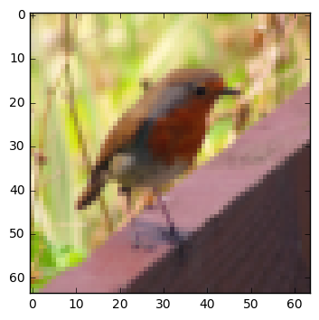
The following code will show you an image in the dataset. Feel free to change the index and re-run the cell multiple times to see other images.

# Example of a picture
index = 10
plt.imshow(train_x_orig[index])
print ("y = " + str(train_y[0,index]) + ". It's a " + classes[train_y[0,index]].decode("utf-8") +  " picture.")

y = 0. It's a non-cat picture.

png

# Explore your dataset 
m_train = train_x_orig.shape[0]
num_px = train_x_orig.shape[1]
m_test = test_x_orig.shape[0]

print ("Number of training examples: " + str(m_train))
print ("Number of testing examples: " + str(m_test))
print ("Each image is of size: (" + str(num_px) + ", " + str(num_px) + ", 3)")
print ("train_x_orig shape: " + str(train_x_orig.shape))
print ("train_y shape: " + str(train_y.shape))
print ("test_x_orig shape: " + str(test_x_orig.shape))
print ("test_y shape: " + str(test_y.shape))

Number of training examples: 209
Number of testing examples: 50
Each image is of size: (64, 64, 3)
train_x_orig shape: (209, 64, 64, 3)
train_y shape: (1, 209)
test_x_orig shape: (50, 64, 64, 3)
test_y shape: (1, 50)

As usual, you reshape and standardize the images before feeding them to the network. The code is given in the cell below.

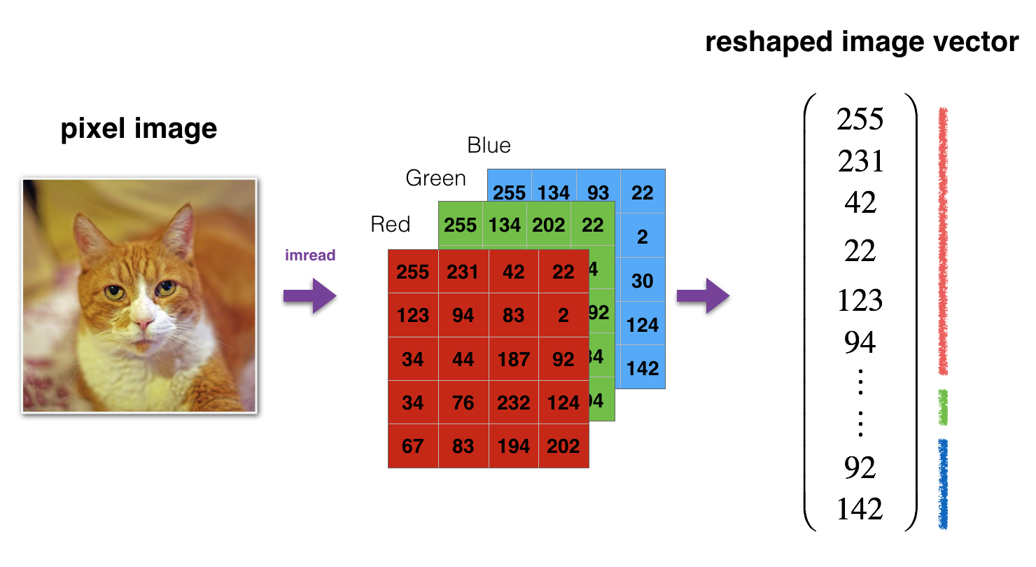
Figure 1: Image to vector conversion.

# Reshape the training and test examples 
train_x_flatten = train_x_orig.reshape(train_x_orig.shape[0], -1).T   # The "-1" makes reshape flatten the remaining dimensions
test_x_flatten = test_x_orig.reshape(test_x_orig.shape[0], -1).T

# Standardize data to have feature values between 0 and 1.
train_x = train_x_flatten/255.
test_x = test_x_flatten/255.

print ("train_x's shape: " + str(train_x.shape))
print ("test_x's shape: " + str(test_x.shape))

train_x's shape: (12288, 209)
test_x's shape: (12288, 50)

$12,288$ equals $64 \times 64 \times 3$ which is the size of one reshaped image vector.

3 - Architecture of your model

Now that you are familiar with the dataset, it is time to build a deep neural network to distinguish cat images from non-cat images.

You will build two different models:

A 2-layer neural network
An L-layer deep neural network

You will then compare the performance of these models, and also try out different values for $L$.

Let’s look at the two architectures.

3.1 - 2-layer neural network

Figure 2: 2-layer neural network.
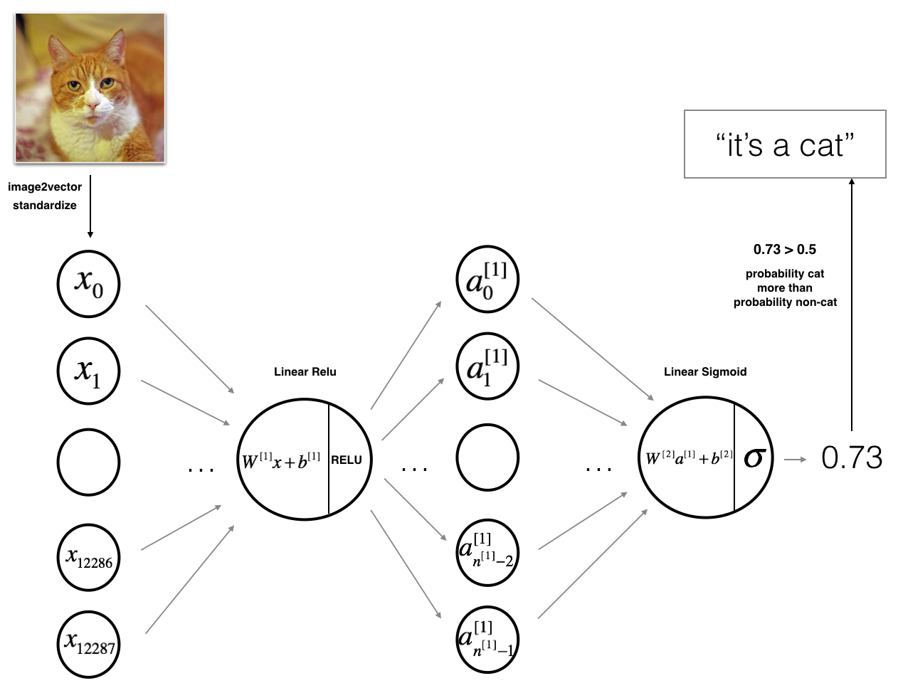
The model can be summarized as: INPUT -> LINEAR -> RELU -> LINEAR -> SIGMOID -> OUTPUT.

Detailed Architecture of figure 2:

The input is a (64,64,3) image which is flattened to a vector of size $(12288,1)$.
The corresponding vector: $[x_0,x_1,…,x_{12287}]^T$ is then multiplied by the weight matrix $W^{[1]}$ of size $(n^{[1]}, 12288)$.
You then add a bias term and take its relu to get the following vector: $[a_0^{[1]}, a_1^{[1]},…, a_{n^{[1]}-1}^{[1]}]^T$.
You then repeat the same process.
You multiply the resulting vector by $W^{[2]}$ and add your intercept (bias).
Finally, you take the sigmoid of the result. If it is greater than 0.5, you classify it to be a cat.

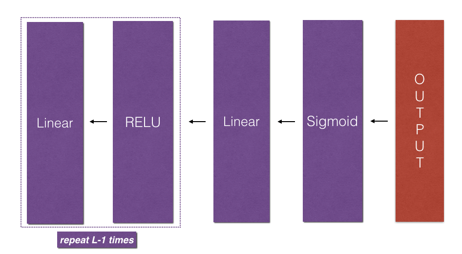
3.2 - L-layer deep neural network

It is hard to represent an L-layer deep neural network with the above representation. However, here is a simplified network representation:

Figure 3: L-layer neural network.
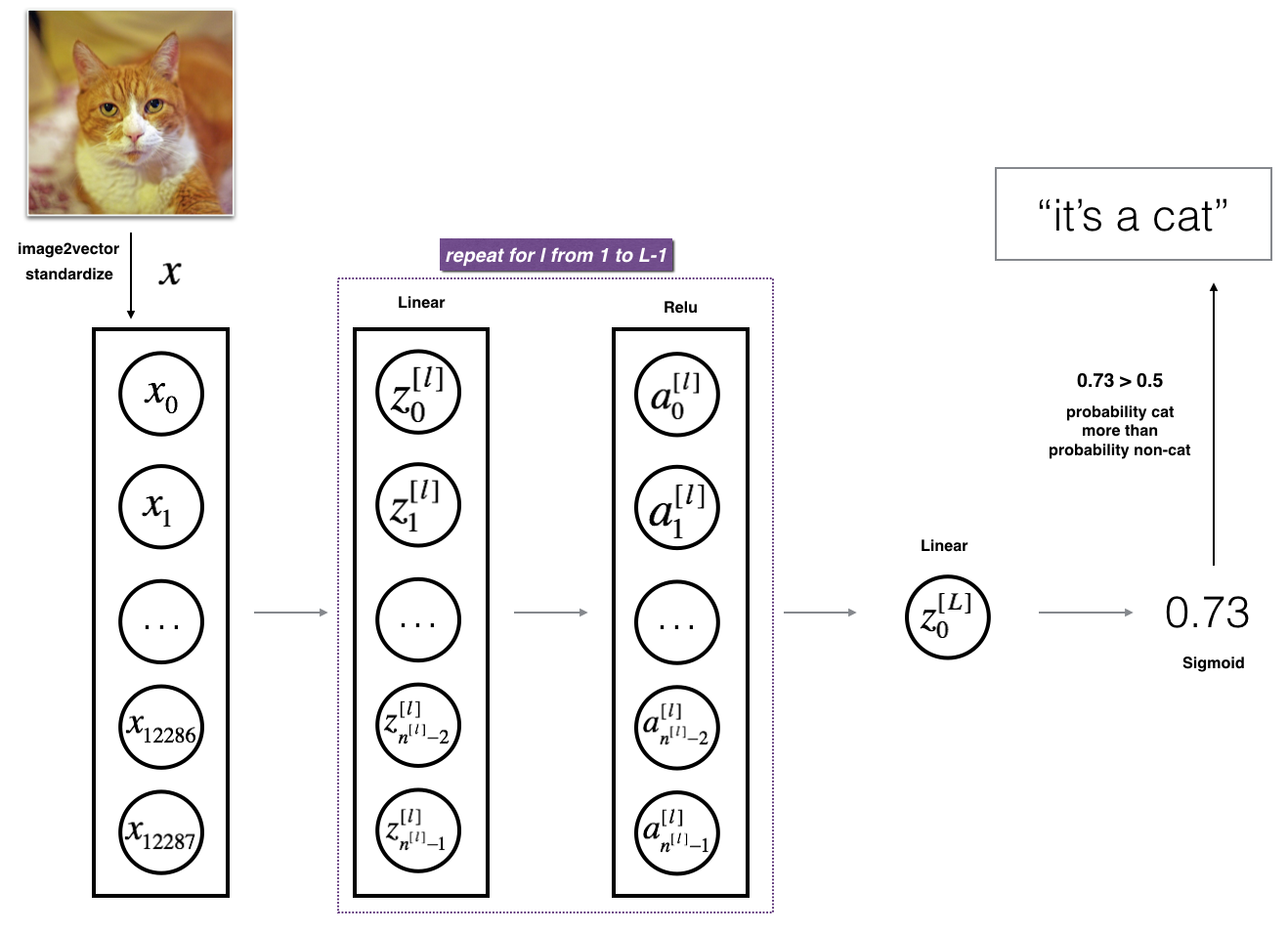
The model can be summarized as: [LINEAR -> RELU] $\times$ (L-1) -> LINEAR -> SIGMOID

Detailed Architecture of figure 3:

The input is a (64,64,3) image which is flattened to a vector of size (12288,1).
The corresponding vector: $[x_0,x_1,…,x_{12287}]^T$ is then multiplied by the weight matrix $W^{[1]}$ and then you add the intercept $b^{[1]}$. The result is called the linear unit.
Next, you take the relu of the linear unit. This process could be repeated several times for each $(W^{[l]}, b^{[l]})$ depending on the model architecture.
Finally, you take the sigmoid of the final linear unit. If it is greater than 0.5, you classify it to be a cat.

3.3 - General methodology

As usual you will follow the Deep Learning methodology to build the model:

1. Initialize parameters / Define hyperparameters
2. Loop for num_iterations:
    a. Forward propagation
    b. Compute cost function
    c. Backward propagation
    d. Update parameters (using parameters, and grads from backprop) 
4. Use trained parameters to predict labels

Let’s now implement those two models!

4 - Two-layer neural network

Question: Use the helper functions you have implemented in the previous assignment to build a 2-layer neural network with the following structure: LINEAR -> RELU -> LINEAR -> SIGMOID. The functions you may need and their inputs are:

def initialize_parameters(n_x, n_h, n_y):
    ...
    return parameters 
def linear_activation_forward(A_prev, W, b, activation):
    ...
    return A, cache
def compute_cost(AL, Y):
    ...
    return cost
def linear_activation_backward(dA, cache, activation):
    ...
    return dA_prev, dW, db
def update_parameters(parameters, grads, learning_rate):
    ...
    return parameters

### CONSTANTS DEFINING THE MODEL ####
n_x = 12288     # num_px * num_px * 3
n_h = 7
n_y = 1
layers_dims = (n_x, n_h, n_y)

# GRADED FUNCTION: two_layer_model

def two_layer_model(X, Y, layers_dims, learning_rate = 0.0075, num_iterations = 3000, print_cost=False):
    """
    Implements a two-layer neural network: LINEAR->RELU->LINEAR->SIGMOID.
    
    Arguments:
    X -- input data, of shape (n_x, number of examples)
    Y -- true "label" vector (containing 0 if cat, 1 if non-cat), of shape (1, number of examples)
    layers_dims -- dimensions of the layers (n_x, n_h, n_y)
    num_iterations -- number of iterations of the optimization loop
    learning_rate -- learning rate of the gradient descent update rule
    print_cost -- If set to True, this will print the cost every 100 iterations 
    
    Returns:
    parameters -- a dictionary containing W1, W2, b1, and b2
    """
    
    np.random.seed(1)
    grads = &#123;&#125;
    costs = []                              # to keep track of the cost
    m = X.shape[1]                           # number of examples
    (n_x, n_h, n_y) = layers_dims
    
    # Initialize parameters dictionary, by calling one of the functions you'd previously implemented
    ### START CODE HERE ### (≈ 1 line of code)
    parameters = initialize_parameters(n_x, n_h, n_y)
    ### END CODE HERE ###
    
    # Get W1, b1, W2 and b2 from the dictionary parameters.
    W1 = parameters["W1"]
    b1 = parameters["b1"]
    W2 = parameters["W2"]
    b2 = parameters["b2"]
    
    # Loop (gradient descent)

    for i in range(0, num_iterations):

        # Forward propagation: LINEAR -> RELU -> LINEAR -> SIGMOID. Inputs: "X, W1, b1, W2, b2". Output: "A1, cache1, A2, cache2".
        ### START CODE HERE ### (≈ 2 lines of code)
        A1, cache1 = linear_activation_forward(X, W1, b1, "relu")
        A2, cache2 = linear_activation_forward(A1, W2, b2, "sigmoid")
        ### END CODE HERE ###
        
        # Compute cost
        ### START CODE HERE ### (≈ 1 line of code)
        cost = compute_cost(A2, Y)
        ### END CODE HERE ###
        
        # Initializing backward propagation
        dA2 = - (np.divide(Y, A2) - np.divide(1 - Y, 1 - A2))
        
        # Backward propagation. Inputs: "dA2, cache2, cache1". Outputs: "dA1, dW2, db2; also dA0 (not used), dW1, db1".
        ### START CODE HERE ### (≈ 2 lines of code)
        dA1, dW2, db2 = linear_activation_backward(dA2, cache2, "sigmoid")
        dA0, dW1, db1 = linear_activation_backward(dA1, cache1, "relu")
        ### END CODE HERE ###
        
        # Set grads['dWl'] to dW1, grads['db1'] to db1, grads['dW2'] to dW2, grads['db2'] to db2
        grads['dW1'] = dW1
        grads['db1'] = db1
        grads['dW2'] = dW2
        grads['db2'] = db2
        
        # Update parameters.
        ### START CODE HERE ### (approx. 1 line of code)
        parameters = update_parameters(parameters, grads, learning_rate)
        ### END CODE HERE ###

        # Retrieve W1, b1, W2, b2 from parameters
        W1 = parameters["W1"]
        b1 = parameters["b1"]
        W2 = parameters["W2"]
        b2 = parameters["b2"]
        
        # Print the cost every 100 training example
        if print_cost and i % 100 == 0:
            print("Cost after iteration &#123;&#125;: &#123;&#125;".format(i, np.squeeze(cost)))
        if print_cost and i % 100 == 0:
            costs.append(cost)
       
    # plot the cost

    plt.plot(np.squeeze(costs))
    plt.ylabel('cost')
    plt.xlabel('iterations (per tens)')
    plt.title("Learning rate =" + str(learning_rate))
    plt.show()
    
    return parameters

Run the cell below to train your parameters. See if your model runs. The cost should be decreasing. It may take up to 5 minutes to run 2500 iterations. Check if the “Cost after iteration 0” matches the expected output below, if not click on the square (⬛) on the upper bar of the notebook to stop the cell and try to find your error.

1	parameters = two_layer_model(train_x, train_y, layers_dims = (n_x, n_h, n_y), num_iterations = 2500, print_cost=True)

Cost after iteration 0: 0.693049735659989
Cost after iteration 100: 0.6464320953428849
Cost after iteration 200: 0.6325140647912678
Cost after iteration 300: 0.6015024920354665
Cost after iteration 400: 0.5601966311605748
Cost after iteration 500: 0.515830477276473
Cost after iteration 600: 0.4754901313943325
Cost after iteration 700: 0.43391631512257495
Cost after iteration 800: 0.4007977536203886
Cost after iteration 900: 0.35807050113237987
Cost after iteration 1000: 0.3394281538366413
Cost after iteration 1100: 0.30527536361962654
Cost after iteration 1200: 0.2749137728213015
Cost after iteration 1300: 0.24681768210614827
Cost after iteration 1400: 0.1985073503746611
Cost after iteration 1500: 0.17448318112556593
Cost after iteration 1600: 0.1708076297809661
Cost after iteration 1700: 0.11306524562164737
Cost after iteration 1800: 0.09629426845937163
Cost after iteration 1900: 0.08342617959726878
Cost after iteration 2000: 0.0743907870431909
Cost after iteration 2100: 0.06630748132267938
Cost after iteration 2200: 0.05919329501038176
Cost after iteration 2300: 0.05336140348560564
Cost after iteration 2400: 0.048554785628770226

png

Expected Output:

Cost after iteration 0	0.6930497356599888
Cost after iteration 100	0.6464320953428849
…	…
Cost after iteration 2400	0.048554785628770206

Good thing you built a vectorized implementation! Otherwise it might have taken 10 times longer to train this.

Now, you can use the trained parameters to classify images from the dataset. To see your predictions on the training and test sets, run the cell below.

1	predictions_train = predict(train_x, train_y, parameters)

Accuracy: 1.0

Expected Output:

Accuracy

1.0

1	predictions_test = predict(test_x, test_y, parameters)

Accuracy: 0.72

Expected Output:

Accuracy

0.72

Note: You may notice that running the model on fewer iterations (say 1500) gives better accuracy on the test set. This is called “early stopping” and we will talk about it in the next course. Early stopping is a way to prevent overfitting.

Congratulations! It seems that your 2-layer neural network has better performance (72%) than the logistic regression implementation (70%, assignment week 2). Let’s see if you can do even better with an $L$-layer model.

5 - L-layer Neural Network

Question: Use the helper functions you have implemented previously to build an $L$-layer neural network with the following structure: [LINEAR -> RELU]$\times$(L-1) -> LINEAR -> SIGMOID. The functions you may need and their inputs are:

def initialize_parameters_deep(layers_dims):
    ...
    return parameters 
def L_model_forward(X, parameters):
    ...
    return AL, caches
def compute_cost(AL, Y):
    ...
    return cost
def L_model_backward(AL, Y, caches):
    ...
    return grads
def update_parameters(parameters, grads, learning_rate):
    ...
    return parameters

1 2	### CONSTANTS ### layers_dims = [12288, 20, 7, 5, 1] # 4-layer model

# GRADED FUNCTION: L_layer_model

def L_layer_model(X, Y, layers_dims, learning_rate = 0.0075, num_iterations = 3000, print_cost=False):#lr was 0.009
    """
    Implements a L-layer neural network: [LINEAR->RELU]*(L-1)->LINEAR->SIGMOID.
    
    Arguments:
    X -- data, numpy array of shape (number of examples, num_px * num_px * 3)
    Y -- true "label" vector (containing 0 if cat, 1 if non-cat), of shape (1, number of examples)
    layers_dims -- list containing the input size and each layer size, of length (number of layers + 1).
    learning_rate -- learning rate of the gradient descent update rule
    num_iterations -- number of iterations of the optimization loop
    print_cost -- if True, it prints the cost every 100 steps
    
    Returns:
    parameters -- parameters learnt by the model. They can then be used to predict.
    """

    np.random.seed(1)
    costs = []                         # keep track of cost
    
    # Parameters initialization. (≈ 1 line of code)
    ### START CODE HERE ###
    parameters = initialize_parameters_deep(layers_dims)
    ### END CODE HERE ###
    
    # Loop (gradient descent)
    for i in range(0, num_iterations):

        # Forward propagation: [LINEAR -> RELU]*(L-1) -> LINEAR -> SIGMOID.
        ### START CODE HERE ### (≈ 1 line of code)
        AL, caches = L_model_forward(X, parameters)
        ### END CODE HERE ###
        
        # Compute cost.
        ### START CODE HERE ### (≈ 1 line of code)
        cost = compute_cost(AL, Y)
        ### END CODE HERE ###
    
        # Backward propagation.
        ### START CODE HERE ### (≈ 1 line of code)
        grads = L_model_backward(AL, Y, caches)
        ### END CODE HERE ###
 
        # Update parameters.
        ### START CODE HERE ### (≈ 1 line of code)
        parameters = update_parameters(parameters, grads, learning_rate)
        ### END CODE HERE ###
                
        # Print the cost every 100 training example
        if print_cost and i % 100 == 0:
            print ("Cost after iteration %i: %f" %(i, cost))
        if print_cost and i % 100 == 0:
            costs.append(cost)
            
    # plot the cost
    plt.plot(np.squeeze(costs))
    plt.ylabel('cost')
    plt.xlabel('iterations (per tens)')
    plt.title("Learning rate =" + str(learning_rate))
    plt.show()
    
    return parameters

You will now train the model as a 4-layer neural network.

Run the cell below to train your model. The cost should decrease on every iteration. It may take up to 5 minutes to run 2500 iterations. Check if the “Cost after iteration 0” matches the expected output below, if not click on the square (⬛) on the upper bar of the notebook to stop the cell and try to find your error.

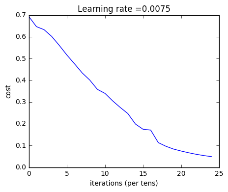
1	parameters = L_layer_model(train_x, train_y, layers_dims, num_iterations = 2500, print_cost = True)

Cost after iteration 0: 0.771749
Cost after iteration 100: 0.672053
Cost after iteration 200: 0.648263
Cost after iteration 300: 0.611507
Cost after iteration 400: 0.567047
Cost after iteration 500: 0.540138
Cost after iteration 600: 0.527930
Cost after iteration 700: 0.465477
Cost after iteration 800: 0.369126
Cost after iteration 900: 0.391747
Cost after iteration 1000: 0.315187
Cost after iteration 1100: 0.272700
Cost after iteration 1200: 0.237419
Cost after iteration 1300: 0.199601
Cost after iteration 1400: 0.189263
Cost after iteration 1500: 0.161189
Cost after iteration 1600: 0.148214
Cost after iteration 1700: 0.137775
Cost after iteration 1800: 0.129740
Cost after iteration 1900: 0.121225
Cost after iteration 2000: 0.113821
Cost after iteration 2100: 0.107839
Cost after iteration 2200: 0.102855
Cost after iteration 2300: 0.100897
Cost after iteration 2400: 0.092878

png

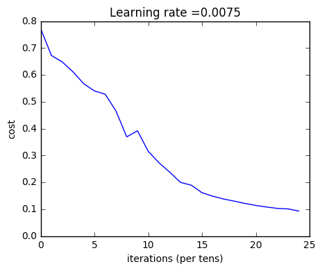
Expected Output:

Cost after iteration 0	0.771749
Cost after iteration 100	0.672053
…	…
Cost after iteration 2400	0.092878

1	pred_train = predict(train_x, train_y, parameters)

Accuracy: 0.985645933014

Train Accuracy

0.985645933014

1	pred_test = predict(test_x, test_y, parameters)

Accuracy: 0.8

Expected Output:

Test Accuracy

0.8

Congrats! It seems that your 4-layer neural network has better performance (80%) than your 2-layer neural network (72%) on the same test set.

This is good performance for this task. Nice job!

Though in the next course on “Improving deep neural networks” you will learn how to obtain even higher accuracy by systematically searching for better hyperparameters (learning_rate, layers_dims, num_iterations, and others you’ll also learn in the next course).

6) Results Analysis

First, let’s take a look at some images the L-layer model labeled incorrectly. This will show a few mislabeled images.

1	print_mislabeled_images(classes, test_x, test_y, pred_test)

png

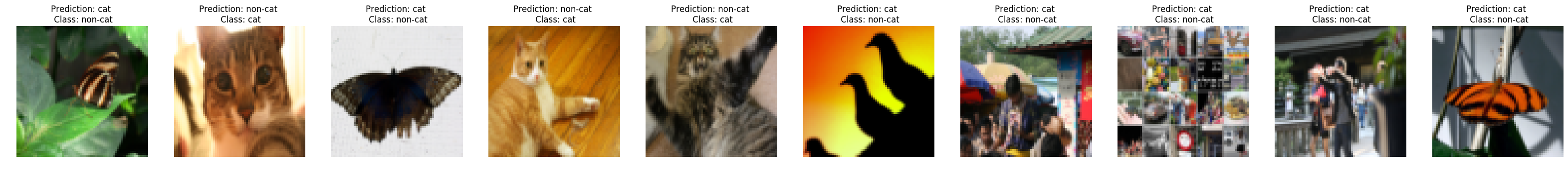
A few types of images the model tends to do poorly on include:

Cat body in an unusual position
Cat appears against a background of a similar color
Unusual cat color and species
Camera Angle
Brightness of the picture
Scale variation (cat is very large or small in image)

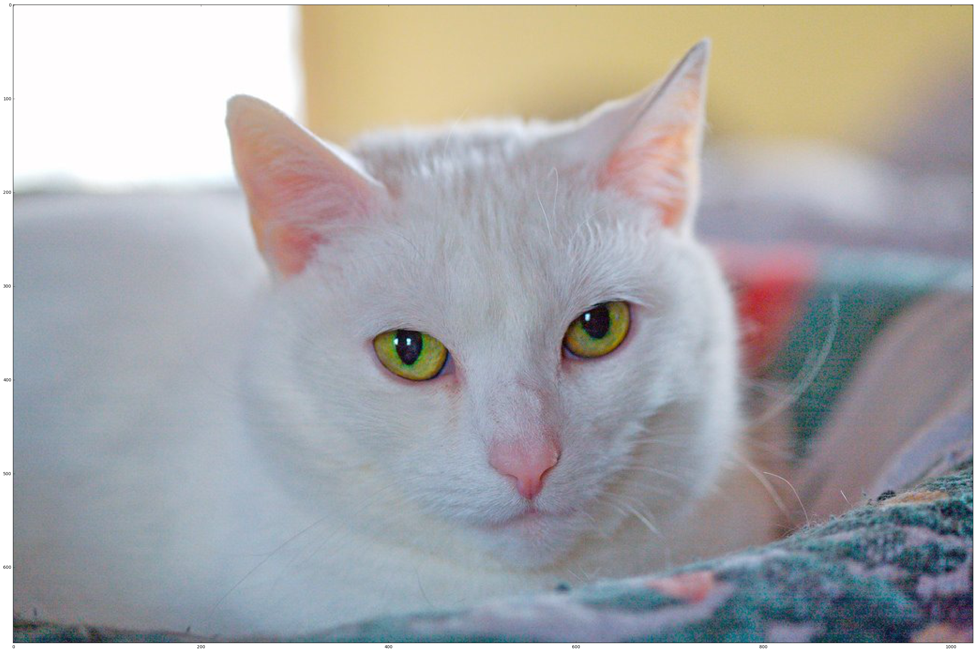
7) Test with your own image (optional/ungraded exercise)

Congratulations on finishing this assignment. You can use your own image and see the output of your model. To do that:

1. Click on "File" in the upper bar of this notebook, then click "Open" to go on your Coursera Hub.
2. Add your image to this Jupyter Notebook's directory, in the "images" folder
3. Change your image's name in the following code
4. Run the code and check if the algorithm is right (1 = cat, 0 = non-cat)!

## START CODE HERE ##
my_image = "my_image.jpg" # change this to the name of your image file 
my_label_y = [1] # the true class of your image (1 -> cat, 0 -> non-cat)
## END CODE HERE ##

fname = "" + my_image
image = np.array(ndimage.imread(fname, flatten=False))
my_image = scipy.misc.imresize(image, size=(num_px,num_px)).reshape((num_px*num_px*3,1))
my_image = my_image/255.
my_predicted_image = predict(my_image, my_label_y, parameters)

plt.imshow(image)
print ("y = " + str(np.squeeze(my_predicted_image)) + ", your L-layer model predicts a \"" + classes[int(np.squeeze(my_predicted_image)),].decode("utf-8") +  "\" picture.")

Accuracy: 1.0
y = 1.0, your L-layer model predicts a "cat" picture.

png

References:

for auto-reloading external module: http://stackoverflow.com/questions/1907993/autoreload-of-modules-in-ipython